How to Calculate Exponential Moving Average using Excel or Google Spreadsheet

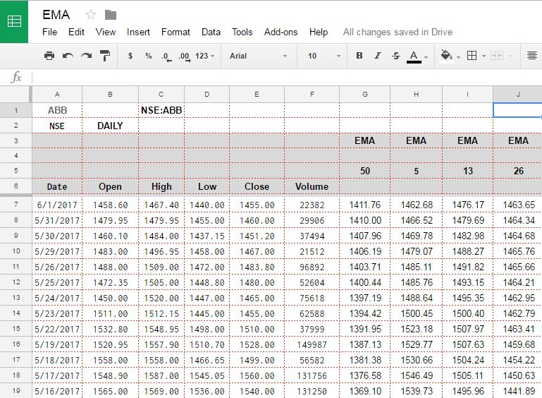
Earlier we told you how to pull historical data in Google spreadsheet (see — HOW TO PULL HISTORICAL STOCK DATA FROM USING GOOGLE SPREADSHEET ) Once you have Historical data available in Google spreadsheet we can calculate Exponential Moving average and values of various technical indicators of our interest using the same.

In this tutorial we going to calculate Exponential Moving Average for given time period using historical data available to us from Google Finance.

EMA or Exponential moving average is also very similar to Simple Moving average, but Simple moving average has little affect of sharp uptrend or Downtrend on current Moving average, to address this issue, Exponential moving average is taken as it gives more weightage to current price or latest price and older prices have less weightage in calculation. Hence EMA moves a little faster when price changes rapidly.

In technical analysis of Share prices, EMA are more popular than Simple Moving average for short term price movement prediction because of this change in way these 2 averages are calculated. Hence Most popular EMA among traders are for short term which are for less than 50 days more specifically 12 days to 26 days EMA prices are generally used based on strategy implemented by Traders.

In case you are interested in learning the mathematics behind calculation of Exponential Moving average you can see — Detailed Mathematical Formula of how EMA is calculated (https://en.wikipedia.org/wiki/Moving_average#Exponential_moving_average)

For EMA Calculation also we will use same trick as we did in SMA, we will enter period for which we need EMA in top column above the values and based on that EMA calculation will be done dynamically. For EMA Calculation we need a seed value, as we usually calculate max 200 EMA, I have provided Seed value in somewhere after 250 ROWS and the formula placed here is the SMA Value of given period. You can also simply put Close price of share as seed value, it won’t affect much if you have lots of data point and well beyond your period of calculation.

Once we have seed values, we can calculate EMA with the help of Standard Exponent function, standard formula for which is = 2/(1+number of periods in MA). You can see the function in Cell just above seed value, for us in excel value it will become = =E252*2/(1+$G$5)+G253*(1-2/(1+$G$5))

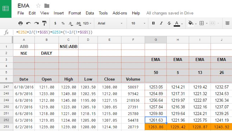
Column E contains Close price for which we calculating EMA, Cell G5 contains period of EMA, which can be changed and formula will be changed dynamically. And G253 is previous value of EMA/SEED value.

Now all we have to do is copy this formula to all cells and we will have EMA value calculated till top.

Link to Google sheet used in this example is — EMA Calculation sheet.